Why PostgreSQL and TimescaleDB Are the Safe Bet for LoRaWAN Data in 2026

The Advice That Aged Badly

For most of the last decade the answer to "where do I put my LoRaWAN data" was easy, and it was InfluxDB. Sensor readings are timestamped measurements, InfluxDB was built for timestamped measurements, and PostgreSQL, asked to hold a few hundred million of them in a plain table, really did get slow. That advice was correct when it was given. The article on this site that gives it is still up, and the stack it describes still works.

Two things have changed since, and they push in the same direction.

The first is that PostgreSQL stopped being bad at this. TimescaleDB is a PostgreSQL extension rather than a fork or a separate server, and it supplies the time-series machinery plain Postgres lacks: automatic partitioning by time, a columnar engine that compresses cold data by up to 98%, materialized views that refresh incrementally instead of recomputing, and retention policies that expire old data on a schedule. The current release, 2.29 from July 2026, runs on PostgreSQL 16, 17 and 18.

The second is that InfluxDB rewrote itself twice, and both rewrites broke the query language.

That combination is why, for most of the LoRaWAN deployments I am asked about in 2026, the recommendation has flipped.

Your Data Was Never Purely Time-Series

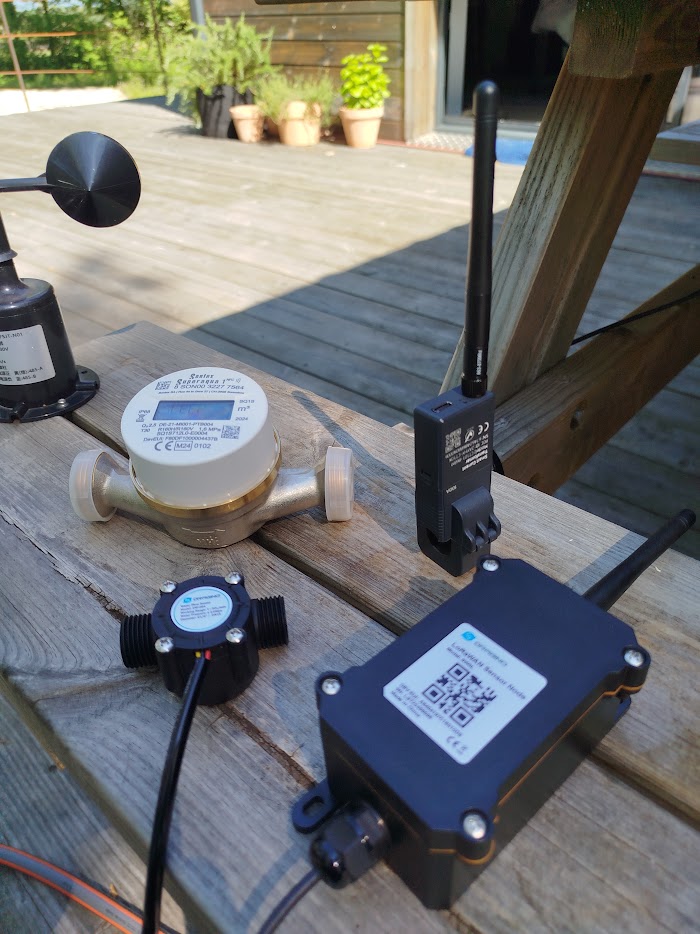
Start with what actually lands in the database, because the framing decides more than any benchmark does.

A LoRaWAN network produces a stream of readings: device, timestamp, value, RSSI, SNR, spreading factor, frame counter. That half is genuinely time-series, and every candidate database handles it competently.

But nothing useful is ever asked of that half alone. The real questions are which site is over budget this month, which tenant owns this meter, which of these readings came from a sensor recalibrated in March, what a building consumed before and after a retrofit, which devices are still under warranty, what the billable total per customer is. Answering any of them means joining measurements against a device registry, a site hierarchy, a tenant table, calibration history, tariffs and installation records. That half is relational, and a time-series database does not do joins.

So the two-database architecture appears. Measurements go to InfluxDB, everything else to Postgres, and the join happens in application code: somebody writes a service that queries one, queries the other, and stitches the results in memory. That service is now what every dashboard depends on, it has to be maintained by whoever inherits it, and it is where the bugs live. Meanwhile Grafana, which could have expressed the whole thing as one SQL query, is reduced to fetching pre-chewed JSON from your own API.

Put both halves in one Postgres and the join is just a join.

Almost every LoRaWAN dashboard that matters is a join between a measurement and a fact about the device that produced it. Choosing storage that cannot express that join means writing the join yourself, forever.

There is a smaller convenience sitting on top of the argument. ChirpStack already runs on PostgreSQL, so the device registry, applications, tenants and device profiles are in there whether you plan around it or not. It also ships a PostgreSQL integration that writes uplink, join, status and error events straight into a database of your choosing, enabled by adding postgresql to the integration list and setting a connection string. On a modest deployment that is the entire ingestion pipeline: no broker consumer to write, no service to keep alive, as covered in the ChirpStack article.

Nobody's LoRaWAN Fleet Is Big

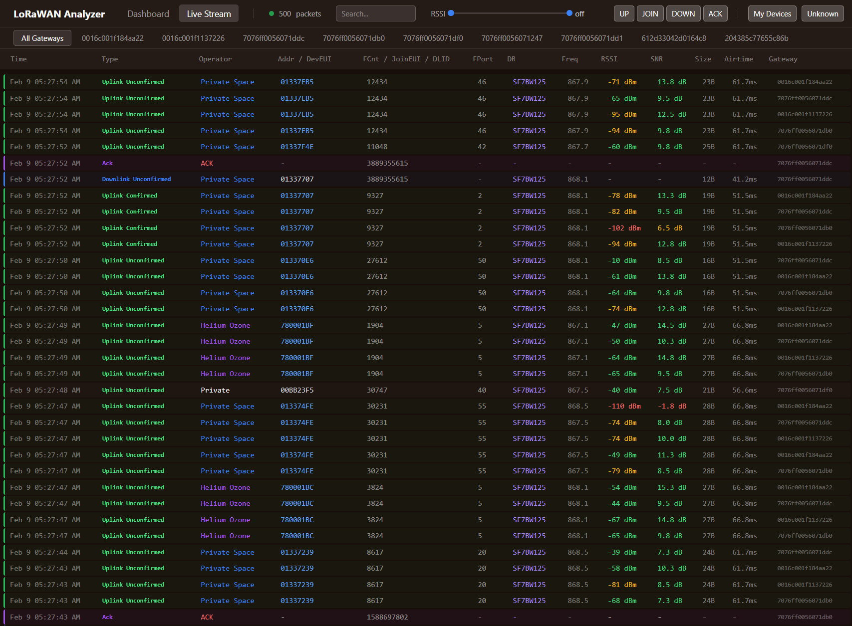
The benchmark arguments between time-series databases are fought over ingest rates in the millions of rows per second. It is worth doing the arithmetic on what a LoRaWAN network actually produces, because the numbers are not close.

A device reporting every fifteen minutes sends 96 uplinks a day, roughly 35,000 a year. Scale that up:

Fleet	Uplinks per day	Rows per year	Sustained rate
500 devices	48,000	17.5 million	0.6/s
2,000 devices	192,000	70 million	2.2/s
10,000 devices	960,000	350 million	11/s
50,000 devices	4.8 million	1.75 billion	56/s

Ten thousand devices is already a large private network, and it works out to about eleven rows per second. That is not a database problem. It is barely a filesystem problem. Any of the candidates ingests it on a small virtual machine without noticing, and unlike an application log it cannot secretly grow by an order of magnitude, because the duty cycle and airtime limits put a hard ceiling on how often a fleet can physically transmit. Counting one row per uplink flatters the numbers, because a schema that stores one row per decoded field multiplies them by the number of values in a payload, typically five or six. Even the 50,000 device line stays comfortably inside what one well-tuned Postgres absorbs.

Which means ingest performance, the thing the benchmarks measure and the vendors argue about, is not the deciding factor for you. What decides it is what you can ask of the data afterwards, and how much work the system will be to keep alive in five years.

What TimescaleDB Actually Adds

Four features do the work, and each one replaces something you would otherwise build by hand.

Hypertables are ordinary tables, transparently partitioned into time-based chunks. You insert and query as though it were a single table, but the planner touches only the chunks overlapping your time range, and indexes stay small because each chunk carries its own. A query for last Tuesday does not read the other four years.

Hypercore is the hybrid storage engine underneath. New rows land in a rowstore, which is what you want for fast inserts and for late uplinks arriving out of order. Once data cools past a threshold you set, it converts to a columnstore, compressing it heavily and making the aggregate queries dashboards actually run substantially faster, since averaging one column no longer means reading twenty. The conversion is a policy, not a cron job somebody has to own.

Continuous aggregates are materialized views that refresh incrementally, recomputing only the time buckets that received new data instead of rescanning the table. This is precisely the downsampling tier every time-series deployment ends up building: raw readings for recent troubleshooting, coarser buckets for the year, coarser still for the decade. The difference is that the view stays live.

Retention policies drop chunks older than a set interval on a schedule, which keeps disk usage flat and predictable rather than quietly climbing until somebody gets paged at 3am.

That is the sales pitch, and it is accurate as far as it goes. What it leaves out is that the shape you give your tables decides whether any of it helps.

Narrow for the Readings, Wide for the Metadata

The features above are the easy part. The shape you give your tables is what decides whether any of them help, and for LoRaWAN that shape is not uniform. The right answer is narrow for one half of the data and wide for the other.

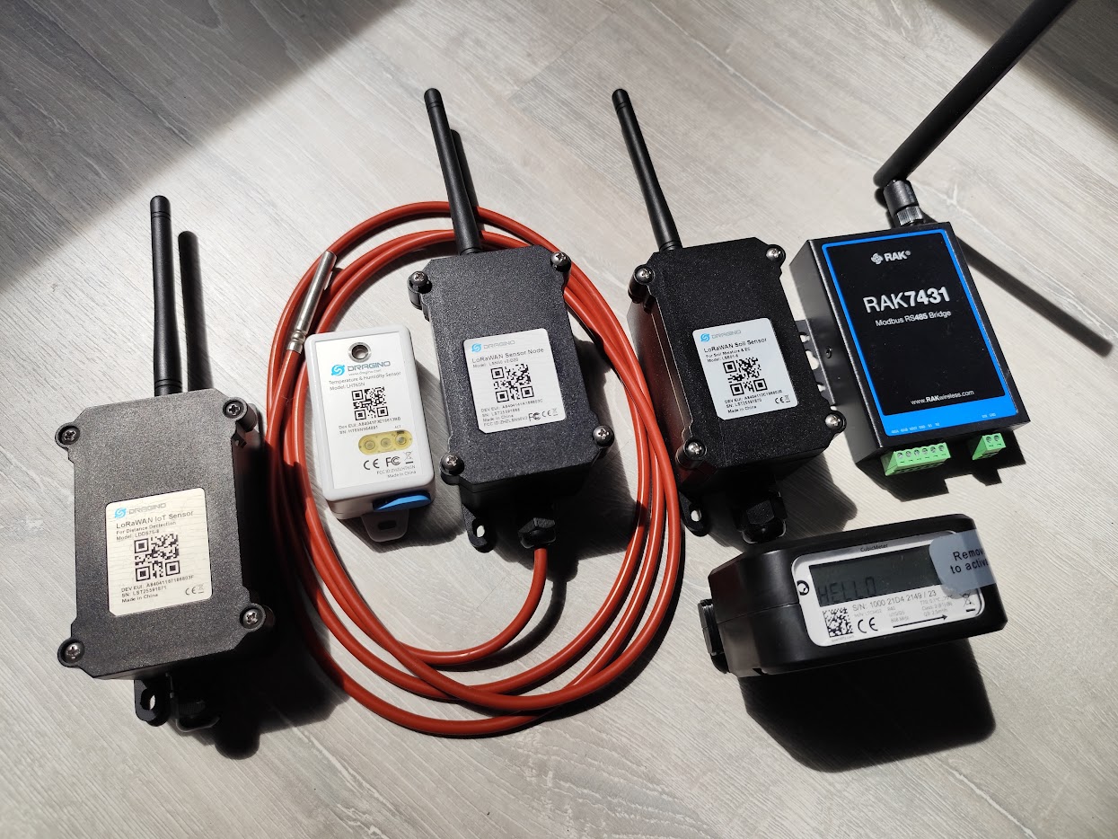
Two hypertables, split by a single question: is this data the same shape on every packet, or not?

An uplinks table is wide. One row per uplink, with real typed columns for everything LoRaWAN itself defines: time, device, network, RSSI, SNR, spreading factor, frame counter, port, frequency, device address, region, the raw payload, which gateways heard it and how many did, and a missed-frame count derived from the counter.

A readings table is narrow. One row per decoded field, with a short fixed set of columns: time, device, field name, value. One uplink becomes as many rows here as its decoder emitted values, which for a typical sensor is five or six.

Why the readings table has to be narrow

The decoded half of the data is heterogeneous and stays that way. Across a mixed fleet, decoders emit hundreds of distinct field names, while any individual device emits a dozen or so of them. That vocabulary is contributed by device vendors rather than by you, and it grows every time somebody integrates a model that reports something new.

A wide table for that is a table with hundreds of columns in which every row populates a dozen. A few percent density, and a schema migration every time the fleet gains a model, each one a deployment window plus a dashboard that has to be taught the new name.

Narrow makes onboarding a sensor a write instead of a schema change. A decoder starts emitting leaf_wetness, it lands in the same table as everything else, and there is no DDL, no downtime, and no coordination needed between whoever wrote the decoder and whoever owns the database.

Storage points the same way. A narrow table is close to the ideal input for a columnar compressor: a low-cardinality field-name column that collapses under dictionary encoding to almost nothing, a device column doing the same, and a value column that is one homogeneous run of doubles. Rows of that shape compress down to a handful of bytes each. The wide, sparse alternative compresses far worse, because every one of those hundreds of columns becomes its own segment, mostly full of NULLs.

Continuous aggregates are where it pays off most visibly. A single aggregate definition grouping by device and field covers every metric you have and every metric you will ever add. The wide equivalent needs an explicit avg() per column, rewritten and backfilled each time a column appears.

The objection, and what the guard rail really looks like

A narrow table is entity-attribute-value, and EAV has a deserved reputation as a relational antipattern. It earns that reputation when it is used to dodge modelling a domain somebody actually understands, trading away types, constraints and foreign keys for a shapeless bag of strings.

The defence is not that the objection is wrong. It is that this particular attribute set is genuinely open, and an open set contributed by third-party vendors is not something anyone could have modelled up front.

What is worth doing is limiting the damage, and the first move is to store the value in several typed columns rather than in one text column holding stringified everything. A float column, a text column and a boolean column, with the populated one carrying the type, means avg() works without a cast, an index on it means something, and a decoder that starts emitting "23.4" instead of 23.4 lands in the wrong column and shows up as missing data rather than silently poisoning a year of averages.

The honest complication is that even this does not fully hold. On any fleet of real size, a handful of field names will disagree about their type from one device to another, arriving as a number from one vendor's decoder and a string from another's. That is simply what a heterogeneous fleet does to a clean data model. It means the useful registry key is not the field name alone but the pairing of device model and field name, and those disagreements are worth hunting down deliberately rather than meeting in a panel that has been quietly plotting a subset of the data.

The map that decides where a field lives

With two tables there has to be one authoritative answer to "where does field X go", and it cannot be a convention people are trusted to remember.

Keep it as a single list in the ingest service: a name on the list becomes a column on the uplinks table, anything not on it becomes a row in readings. The map runs at write time, which is the part that matters. A name written to one table and looked for in the other is simply unreadable, with no error and no empty result to tip you off, just a panel that has always been blank and that nobody can explain. Treat adding to that list as a schema change, and have the query layer derive its behaviour from the same map rather than from somebody's memory of it.

The rollup cascade, and why it stores sums

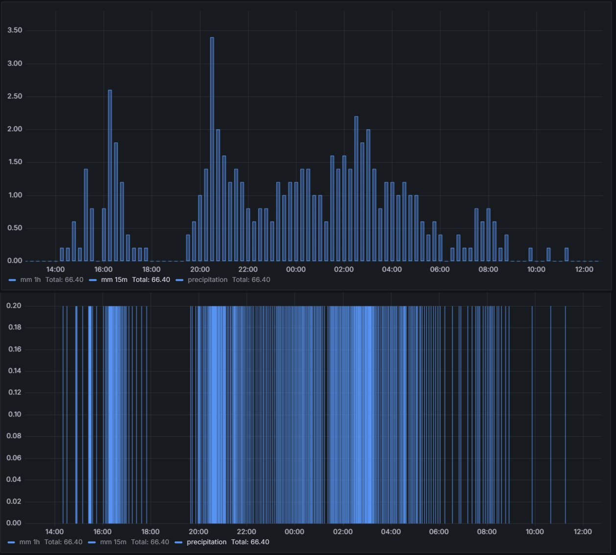
Downsampling wants more than one tier, and the tiers should be built on each other rather than all of them on the raw table. Five-minute buckets over the raw readings, thirty-minute buckets over the five-minute ones, three-hour buckets over those. Each refresh then reads a handful of rows from the tier below instead of rescanning millions of raw ones, and each tier lands several times smaller than the one beneath it, so the whole cascade costs a fraction of what the raw data does.

Store bucket, device, field, sum, count, min, max. The detail that matters is that it stores a sum and a count, never a mean. Rolling one tier into the next is then sum(sum) / sum(count), which is the true average of the underlying readings.

Storing a mean would look simpler and be wrong. Averaging averages weights every bucket equally regardless of how many readings went into it, so a five-minute window holding one reading counts as much as one holding sixty, and a device that dropped most of an hour quietly drags the hourly figure toward its few surviving samples. The error is small enough to pass review and large enough to matter on a billing report. Sum and count is the only shape that composes, which is also why min and max are stored and a median is not.

The join the whole article rests on then reads from whichever tier suits the range:

SELECT s.name AS site,
       r.bucket,
       sum(r.sum_f) / sum(r.n) AS temperature
FROM readings_30m r
JOIN device d ON d.id = r.device
JOIN site   s ON s.id = d.site_id
WHERE r.field = 'temperature'
  AND r.bucket >= '2026-07-01'
  AND r.bucket <  '2026-08-01'
  AND s.tenant_id = $1
GROUP BY s.name, r.bucket;

Grafana runs that directly against its PostgreSQL data source. The site name and the tenant scoping come from tables that are the system of record rather than from strings copied into measurement tags and left to drift.

Two things that will bite you

Both are the kind of thing you learn exactly once.

Bound every query with a literal the caller computed. Chunk exclusion happens at plan time, so the planner has to be able to see the time range before it runs anything. That is why the query above uses two hard dates rather than the more natural now() - INTERVAL '30 days'. Give the planner a visible range and it opens only the chunks that matter; leave the bound open, or hide it behind an expression it cannot fold, and it plans a scan of the entire hypertable. On compressed chunks that is not merely slow, it is catastrophic, because every segment has to be decompressed before it can be examined. This is the most common reason a TimescaleDB deployment that was quick in testing is not quick in production.

Read the cascade only below its watermark. Real-time aggregation, where a continuous aggregate transparently unions its materialised buckets with raw rows arriving after them, does not compose across a cascade. A parent tier that has fallen behind does not return missing buckets, which you would notice immediately. It returns short ones, computed from however much of the child it has materialised so far, and a short bucket looks exactly like a genuine dip in the data. Query each tier only up to the point it has actually materialised, and fall back to the tier below for anything more recent than that.

A packet is not a row

One consequence surprises people, so it is worth stating outright: nothing in this design stores a packet. The radio metadata is in one table, the decoded values are spread across several rows of another, and reconstructing an uplink as a single object means joining uplinks to a pivot of readings.

That is a deliberate trade. Reassembling one packet is a query you write occasionally, usually while debugging a decoder. Charting one field across a fleet for a month, or joining a reading to the device that produced it, is a query the system runs thousands of times a day. The schema is shaped for the second one, on purpose.

The Migration Tax

The second half of the argument is not about capability at all. It is about how much rework a storage choice imposes over the life of a deployment, and LoRaWAN infrastructure gets specified once and then runs for years, frequently on sites nobody wants to revisit. Churn in the data layer is disproportionately expensive here.

InfluxDB has now shipped three major versions that do not share a query language. Version 1 spoke InfluxQL over the TSM engine. Version 2 introduced Flux, and a great many dashboards were written in it. Version 3 is a ground-up rewrite from Go to Rust on Apache Arrow and Parquet, and Flux could not make the journey: it sits in maintenance mode receiving security patches and critical fixes but no development, and InfluxDB 3 does not support it. Anyone who invested in Flux between 2020 and 2023 is rewriting those queries in SQL or InfluxQL to move forward. The new engine is good and the rewrite was defensible engineering. The cost still landed on the operator.

There is a second detail that matters specifically for self-hosted work. InfluxDB 3 Core, the free open-source edition, limits a single query to a 72-hour span. The cap comes from a default limit of 432 Parquet files per query plan, and while it is configurable, raising it drives memory consumption up with it, because Core is deliberately built as a recent-data engine. Querying longer ranges is one of the capabilities reserved for the paid Enterprise tier, which is at least now free for at-home and non-commercial use.

For plenty of workloads that split is reasonable. For LoRaWAN it is awkward, because nearly every question that justifies the deployment is a long-range one: this winter against last winter, consumption before and after the retrofit, a season of irrigation patterns, a year of billing. A free tier that answers "the last three days" well is not aimed at what you are building.

Against that, SQL written over a Timescale hypertable is ordinary PostgreSQL. It survives major version upgrades, it is understood by every reporting tool, BI product and ORM your client already owns, and there is no bespoke query language that can be put into maintenance mode. That is a boring property, and it is the entire point.

Being Fair About It

None of this makes InfluxDB a bad database or a mistake to be running.

If you already have an InfluxDB deployment doing its job, migrating for its own sake is wasted budget and I will say so. InfluxDB 3 is genuinely fast, its Parquet-on-object-storage design is a good fit if you want cheap unlimited retention on S3-compatible storage, and a team fluent in InfluxQL has a real reason to stay put.

There are also cases where neither tool is the answer. Genuinely high-frequency data, vibration or acoustic waveforms sampled in kilohertz, is a different engineering problem, and it does not arrive over LoRaWAN in the first place. If a deployment is already committed to a cloud provider's native services, the Azure IoT Hub and AWS IoT Core route is often a shorter path than running storage yourself. And for pure infrastructure metrics rather than sensor readings, Prometheus fits better than either.

One point belongs in procurement rather than in an audit. TimescaleDB's core is Apache 2.0, but the features this article is built on, the compression, the continuous aggregates and the policies, are community edition under the Timescale License. That license is source-available and free to use, including commercially, with a single restriction that binds only if you intend to resell it as a hosted database service. For anyone deploying it for their own use or a client's it costs nothing, but it is not OSI open source, and it is better to know that before somebody asks.

What It Looks Like Deployed

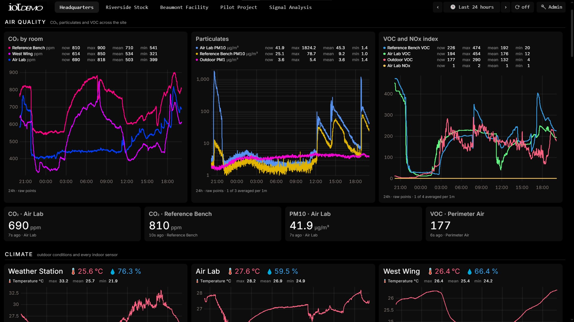
The dashboard at the top of this page is what that schema looks like from the front. It is the live demo linked throughout this site: real devices reporting air quality, climate and signal quality, with every panel backed by SQL against those tables rather than by a service stitching two databases together. The 24 hour view you land on is served from raw rows, longer ranges come from the cascade, and that is the only reason the page stays quick as the history grows.

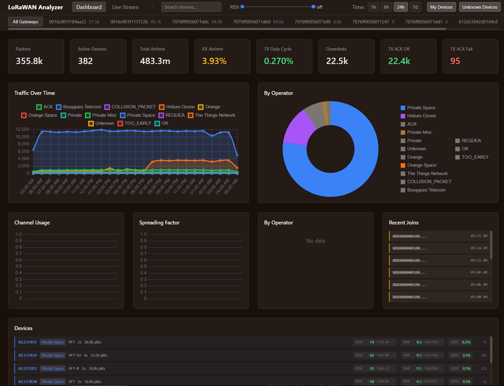
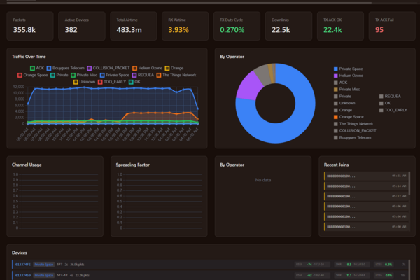
The LoRaWAN traffic analyzer puts the same storage to a different job, capturing every gateway event on the air and keeping millions of packets queryable for congestion analysis. It ships as two containers, the analyzer and a Postgres with TimescaleDB, which is a fair measure of how much operational weight this adds: one more container, and it is the same Postgres your team already knows how to back up.

That last point usually decides the argument on a real project. Postgres backup, replication, monitoring, connection pooling and access control are solved problems with a deep bench of people who know them, and a client's existing operations team has almost certainly run one before. A dedicated time-series database is one more distinct system for whoever is on call to learn, at 3am, from documentation.

What I Provide

The storage layer tends to get chosen in an afternoon and then lived with for a decade, usually by whoever is closest to the dashboard rather than by whoever will be maintaining it in 2031. It is worth more thought than it gets.

I design and deploy the data layer under LoRaWAN networks: schema design that keeps the relational and time-series halves in one place, the ingestion path from your network server, continuous aggregate tiers and retention policies sized against what you actually query rather than what you might, and the Grafana or custom dashboards reading from them. Where an existing InfluxDB deployment is working, I will tell you to keep it and spend the money on something that needs it. Where it is being outgrown, or heading into a version migration nobody planned for, I handle the move including the historical data.

Everything is self-hosted on infrastructure you own, and everything is handed over: schema and migrations, ingestion code, dashboard definitions, and the documentation to run all of it. No licensing fees, no recurring platform cost, and no dependency on me once it is running.